User guide · 2.0

Notebook 3 - Python Workflows

In this notebook, you’ll learn how SHOTpy fits into a broader Python ecosystem (e.g., by using NumPy, pandas, matplotlib, SciPy, machine learning pipelines, data pipelines).

Table of Contents

0. Setup

1. Bin Packing Problem

   1.1. Load Problem Data

   1.2. Build and Solve Model

   1.3. Visualize and Analyze Results

   1.4. Callback-Based Extension

2. Notebook 3 - Key Takeaways

0. Setup

First, install SHOTpy and the Python libraries used in this notebook, then import them.

%pip install SHOTpy pandas matplotlib

import SHOTpy

import matplotlib.pyplot as plt
import numpy as np
import pandas as pd
from IPython.display import HTML, display
from mpl_toolkits.mplot3d.art3d import Poly3DCollection

1. Bin Packing Problem

The Bin Packing Problem (BPP) is a classic combinatorial optimization problem: given a set of items (boxes, packages, …), each with a certain size (width × depth × height), pack them all into the fewest possible bins without exceeding each bin’s capacity.

Each item can be rotated by 90° about the axes, so it can be placed in any of the 6 permutations of its dimensions (W, D, H), selected by binary variables. The objective is linear in the number of bins and quadratic in the positions of the items, so the problem is a convex mixed-integer quadratic problem.

Sets

• \(I\): Set of items, indexed by \(i\)

• \(J\): Set of potential bins, indexed by \(j\)

• \(P = \{0,\dots,5\}\): Set of orientation indices (the 6 axis-aligned permutations of W, D, H)

Parameters

• \(w_i, d_i, h_i\): Width, depth, height of item \(i \in I\) in its canonical orientation

• \(W, D, H\): Bin dimensions

• \(M\): Big-M

• \(\lambda\): Large positive penalty coefficient used to bias the optimization toward solutions with fewer bins

• \((\alpha_p, \beta_p, \gamma_p)\): Effective (width, depth, height) multipliers for permutation \(p \in P\), drawn from the 6 permutations of \((w_i, d_i, h_i)\): $\( \begin{array}{c|ccc} p & \alpha & \beta & \gamma \\ \hline 0 & w & d & h \\ 1 & w & h & d \\ 2 & d & w & h \\ 3 & d & h & w \\ 4 & h & w & d \\ 5 & h & d & w \end{array} \)$

Variables

Bin assignments

• \(x_{ij} \in \{0,1\}\): 1 if item \(i\) is assigned to bin \(j\)

• \(y_j \in \{0,1\}\): 1 if bin \(j\) is used

Item placement

• \(X_i, Y_i, Z_i \ge 0\): Coordinates of the lower-left-front corner of item \(i\)

Orientation (axis-aligned, binary)

• \(r_{ip} \in \{0,1\}\): 1 if item \(i\) uses permutation \(p\)
  Exactly one permutation is active: \(\sum_{p} r_{ip} = 1\)

Effective dimensions (auxiliary continuous, linearise the product \(r_{ip} \cdot \text{dim}\))

• \(\tilde{w}_i, \tilde{d}_i, \tilde{h}_i \ge 0\): Effective width, depth, height of item \(i\) after orientation selection

\[\tilde{w}_i = \sum_{p} \alpha_p^i\, r_{ip}, \quad \tilde{d}_i = \sum_{p} \beta_p^i\, r_{ip}, \quad \tilde{h}_i = \sum_{p} \gamma_p^i\, r_{ip}\]

Relative positioning

For every pair of items \(i < k\):

• \(L_{ik}, R_{ik}, F_{ik}, B_{ik}, U_{ik}, D_{ik} \in \{0,1\}\): Six separation indicators (left/right/front/behind/below/above)

Model $$

(1)\[\begin{align} \min \quad & \lambda\sum_{j \in J} y_j + \sum_{i \in I} (X_i^2 + Y_i^2 + Z_i^2) && \text{(minimize number of bins while preferring compact item placement to one corner)} \\[6pt] \text{s.t.} \quad & \sum_{j \in J} x_{ij} = 1, \quad \forall i \in I && \text{(each item assigned to exactly one bin)} \\[6pt] & x_{ij} \le y_j, \quad \forall i \in I,\; j \in J && \text{(bin must be open if used)} \\[6pt] & \sum_{p \in P} r_{ip} = 1, \quad \forall i \in I && \text{(exactly one orientation per item)} \\[6pt] & X_i + \tilde{w}_i \le W + M(1-x_{ij}), \quad \forall i \in I,\; j \in J && \text{(item fits within bin width)} \\ & Y_i + \tilde{d}_i \le D + M(1-x_{ij}), \quad \forall i \in I,\; j \in J && \text{(item fits within bin depth)} \\ & Z_i + \tilde{h}_i \le H + M(1-x_{ij}), \quad \forall i \in I,\; j \in J && \text{(item fits within bin height)} \\[6pt] & X_i + \tilde{w}_i \le X_k + M(1-L_{ik}), \quad \forall i < k && \text{(item $i$ left of item $k$)} \\ & X_k + \tilde{w}_k \le X_i + M(1-R_{ik}), \quad \forall i < k && \text{(item $i$ right of item $k$)} \\ & Y_i + \tilde{d}_i \le Y_k + M(1-F_{ik}), \quad \forall i < k && \text{(item $i$ in front of item $k$)} \\ & Y_k + \tilde{d}_k \le Y_i + M(1-B_{ik}), \quad \forall i < k && \text{(item $i$ behind item $k$)} \\ & Z_i + \tilde{h}_i \le Z_k + M(1-U_{ik}), \quad \forall i < k && \text{(item $i$ below item $k$)} \\ & Z_k + \tilde{h}_k \le Z_i + M(1-D_{ik}), \quad \forall i < k && \text{(item $i$ above item $k$)} \\[6pt] & L_{ik}+R_{ik}+F_{ik}+B_{ik}+U_{ik}+D_{ik} \ge x_{ij}+x_{kj}-1, \quad \forall i < k,\; j \in J && \text{(items in same bin must be separated)} \\[6pt] & x_{ij},\, y_j,\, r_{ip} \in \{0,1\} \\ & L_{ik},\,R_{ik},\,F_{ik},\,B_{ik},\,U_{ik},\,D_{ik} \in \{0,1\} \\ & \tilde{w}_i,\, \tilde{d}_i,\, \tilde{h}_i \ge 0 \end{align}\]

$$

1.1. Load Problem Data

Item data is stored in binpacking_items.csv. We begin by loading it with pandas, and computing a few useful statistics.

# Load item data
df = pd.read_csv("binpacking_items.csv")
df["volume"] = df["width"] * df["depth"] * df["height"]

# Display a styled table
display(HTML(df.to_html(index=False)))

# Item set and item data
I = df["item_id"].tolist()
widths = dict(zip(I, df["width"].tolist()))
depths = dict(zip(I, df["depth"].tolist()))
heights = dict(zip(I, df["height"].tolist()))
volumes = dict(zip(I, df["volume"].tolist()))

# Potential bins (worst case: one bin per item)
J = list(range(len(I)))

# Bin dimensions
BIN_WIDTH, BIN_DEPTH, BIN_HEIGHT = 12, 10, 10
BIN_VOLUME = BIN_WIDTH * BIN_DEPTH * BIN_HEIGHT

# Summary statistics
print(f"Number of items   : {len(I)}")
print(f"Total item volume : {sum(volumes.values())}")
print(f"Bin dimensions    : {BIN_WIDTH} × {BIN_DEPTH} × {BIN_HEIGHT}")
print(f"Bin volume        : {BIN_VOLUME}")

item_id	width	depth	height	volume
I001	10	8	5	400
I002	4	6	3	72
I003	12	7	4	336
I004	5	5	5	125
I005	3	6	7	126
I006	6	10	5	300
I007	7	4	10	280
I008	2	2	8	32
I009	2	2	6	24
I010	6	10	4	240

Number of items   : 10
Total item volume : 1935
Bin dimensions    : 12 × 10 × 10
Bin volume        : 1200

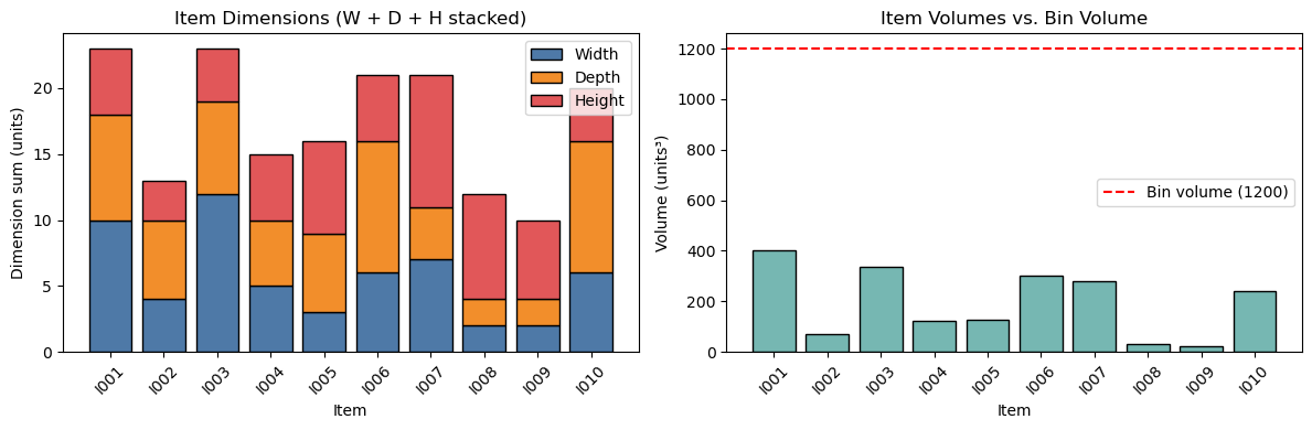
Before jumping into optimization, let’s use matplotlib to get a feel for the item size distribution.

fig, axes = plt.subplots(1, 2, figsize=(12, 4))

x_pos = np.arange(len(I))
w_vals = [widths[i] for i in I]
d_vals = [depths[i] for i in I]
h_vals = [heights[i] for i in I]

# Stacked bar: width / depth / height per item
axes[0].bar(x_pos, w_vals, label='Width', color='#4E79A7', edgecolor='black')
axes[0].bar(x_pos, d_vals, bottom=w_vals, label='Depth', color='#F28E2B', edgecolor='black')
axes[0].bar(x_pos, h_vals, bottom=np.add(w_vals, d_vals), label='Height', color='#E15759', edgecolor='black')
axes[0].set_xticks(x_pos)
axes[0].set_xticklabels(I, rotation=45)
axes[0].set_xlabel('Item')
axes[0].set_ylabel('Dimension sum (units)')
axes[0].set_title('Item Dimensions (W + D + H stacked)')
axes[0].legend()

# Item volumes vs. bin volume
axes[1].bar(x_pos, [volumes[i] for i in I], color='#76B7B2', edgecolor='black')
axes[1].axhline(y=BIN_VOLUME, color='red', linestyle='--', label=f'Bin volume ({BIN_VOLUME})')
axes[1].set_xticks(x_pos)
axes[1].set_xticklabels(I, rotation=45)
axes[1].set_xlabel('Item')
axes[1].set_ylabel('Volume (units³)')
axes[1].set_title('Item Volumes vs. Bin Volume')
axes[1].legend()

plt.tight_layout()
plt.show()

1.2. Build and Solve Model

Now let’s build the bin packing model in SHOTpy. The structure follows the same pattern established in Notebook 1: create solver → create problem → add variables, objective and constraints → finalize problem → set problem → solve.

Since we solve the same model again in Section 1.4, the model is built by a function, build_binpacking_model(solver), which returns the finalized problem and its variables. The constraints are written as comparisons that follow the model above, e.g., X[i] + w_eff[i] <= BIN_WIDTH + M * (1 - x[i, j]), where w_eff[i] is the effective width \(\tilde{w}_i\).

# Big-M (>= largest possible effective dimension in any orientation)
M = BIN_WIDTH + BIN_DEPTH + BIN_HEIGHT

# Lambda for objective weighting: prioritise bin count over compact placement
LAMBDA = 1000

# Orientation permutations: the 6 axis-aligned 90° rotations. Each row gives (eff_width, eff_depth, eff_height)
# as indices into (w_i, d_i, h_i), where 0 = w, 1 = d, 2 = h
PERM_DIMS = [
    (0, 1, 2),  # p=0: (w, d, h)  — identity
    (0, 2, 1),  # p=1: (w, h, d)
    (1, 0, 2),  # p=2: (d, w, h)
    (1, 2, 0),  # p=3: (d, h, w)
    (2, 0, 1),  # p=4: (h, w, d)
    (2, 1, 0),  # p=5: (h, d, w)
]
P = list(range(len(PERM_DIMS)))
PERM_LABELS = ["(W,D,H)", "(W,H,D)", "(D,W,H)", "(D,H,W)", "(H,W,D)", "(H,D,W)"]

# Pairs of items i < k
pairs = [(I[a], I[b]) for a in range(len(I)) for b in range(a + 1, len(I))]


def eff_dims(item, p):
    """Return (eff_w, eff_d, eff_h) for the item in orientation p."""
    src = [widths[item], depths[item], heights[item]]
    a, b, g = PERM_DIMS[p]
    return src[a], src[b], src[g]


def build_binpacking_model(solver):
    """Create the bin packing problem; returns the finalized problem and a dict with its variables."""
    problem = SHOTpy.Problem(solver)
    Binary, Real = SHOTpy.VariableType.Binary, SHOTpy.VariableType.Real

    # ── Variables ────────────────────────────────────────────────────────────────
    # x[i, j]          = 1 if item i is placed in bin j
    # y[j]             = 1 if bin j is used
    # X[i], Y[i], Z[i] = coordinates of the lower-left-front corner of item i
    # r[i, p]          = 1 if item i uses orientation p
    # sep[s, i, k]     = 1 if item i is left/right/in front of/behind/below/above (s = L/R/F/B/U/D) item k, i < k
    x = {(i, j): problem.addVariable(f"x_{i}_{j+1}", Binary) for i in I for j in J}
    y = {j: problem.addVariable(f"y_{j+1}", Binary) for j in J}

    X, Y, Z, r = {}, {}, {}, {}
    for i in I:
        X[i] = problem.addVariable(f"X_{i}", Real, 0, BIN_WIDTH)
        Y[i] = problem.addVariable(f"Y_{i}", Real, 0, BIN_DEPTH)
        Z[i] = problem.addVariable(f"Z_{i}", Real, 0, BIN_HEIGHT)
        for p in P:
            r[i, p] = problem.addVariable(f"r_{i}_{p}", Binary)

    sep = {(s, i, k): problem.addVariable(f"{s}_{i}_{k}", Binary) for (i, k) in pairs for s in "LRFBUD"}

    # Effective dimensions of each item, linear in the orientation variables r[i, p]
    w_eff = {i: sum(eff_dims(i, p)[0] * r[i, p] for p in P) for i in I}
    d_eff = {i: sum(eff_dims(i, p)[1] * r[i, p] for p in P) for i in I}
    h_eff = {i: sum(eff_dims(i, p)[2] * r[i, p] for p in P) for i in I}

    # ── Objective: minimize the number of bins, then prefer compact placement in one corner ──
    problem.setObjective(LAMBDA * sum(y[j] for j in J) + sum(X[i]**2 + Y[i]**2 + Z[i]**2 for i in I),
                         SHOTpy.ObjectiveDirection.Minimize)

    # ── Constraints ──────────────────────────────────────────────────────────────
    # Each item assigned to exactly one bin
    for i in I:
        problem.addConstraint(sum(x[i, j] for j in J) == 1, f"assign_{i}")

    # Bin must be open if used
    for i in I:
        for j in J:
            problem.addConstraint(x[i, j] <= y[j], f"open_{i}_{j+1}")

    # Exactly one orientation per item
    for i in I:
        problem.addConstraint(sum(r[i, p] for p in P) == 1, f"orient_{i}")

    # Item fits within the bin
    for i in I:
        for j in J:
            problem.addConstraint(X[i] + w_eff[i] <= BIN_WIDTH + M * (1 - x[i, j]), f"fit_w_{i}_{j+1}")
            problem.addConstraint(Y[i] + d_eff[i] <= BIN_DEPTH + M * (1 - x[i, j]), f"fit_d_{i}_{j+1}")
            problem.addConstraint(Z[i] + h_eff[i] <= BIN_HEIGHT + M * (1 - x[i, j]), f"fit_h_{i}_{j+1}")

    # Non-overlap for every pair of items i < k
    for (i, k) in pairs:
        problem.addConstraint(X[i] + w_eff[i] <= X[k] + M * (1 - sep["L", i, k]), f"left_{i}_{k}")
        problem.addConstraint(X[k] + w_eff[k] <= X[i] + M * (1 - sep["R", i, k]), f"right_{i}_{k}")
        problem.addConstraint(Y[i] + d_eff[i] <= Y[k] + M * (1 - sep["F", i, k]), f"front_{i}_{k}")
        problem.addConstraint(Y[k] + d_eff[k] <= Y[i] + M * (1 - sep["B", i, k]), f"behind_{i}_{k}")
        problem.addConstraint(Z[i] + h_eff[i] <= Z[k] + M * (1 - sep["U", i, k]), f"below_{i}_{k}")
        problem.addConstraint(Z[k] + h_eff[k] <= Z[i] + M * (1 - sep["D", i, k]), f"above_{i}_{k}")

        # Items in the same bin must be separated in at least one direction
        for j in J:
            problem.addConstraint(sum(sep[s, i, k] for s in "LRFBUD") >= x[i, j] + x[k, j] - 1, f"sep_{i}_{k}_{j+1}")

    # Symmetry breaking: bin j can only be used if bin j-1 is used
    for j in range(1, len(J)):
        problem.addConstraint(y[j] <= y[j - 1], f"sym_{j+1}")

    problem.finalize()
    return problem, {"x": x, "y": y, "X": X, "Y": Y, "Z": Z, "r": r}

A note on solve time: Proving that a packing is optimal is much harder than finding a good one. With HiGHS, SHOT finds a packing into two bins within a second, but closing the gap to the dual bound takes far longer. We therefore stop the solve after 60 seconds with Termination.TimeLimit and use the best packing found so far; the status is then FeasibleSolution rather than OptimalGlobal.

# Create solver
solver = SHOTpy.Solver()
solver.updateSetting("Dual.MIP.Solver", int(SHOTpy.MIPSolver.Highs))   # Gurobi, Cplex, Cbc or Highs
solver.updateSetting("Termination.TimeLimit", 60.0)                     # Stop after 60 s with the best packing found

# Create problem
problem, variables = build_binpacking_model(solver)

# Set problem
assert solver.setProblem(problem)

# Solve
assert solver.solveProblem()

 Performing bound tightening on original problem.
  - Bounds for 0 variables tightened in 0.00 s and 1 passes.
  - Objective bounds are: [0, 13440]

 Performing bound tightening on reformulated problem.
  - Bounds for 0 variables tightened in 0.00 s and 1 passes.
  - Objective bounds are: [0, 13440]
- Interior point search ──────────────────────────────────────────────────────────────────────────────────────────────╴

 Strategy selected:          cutting plane minimax
    Iteration     │  Time  │    Cuts     │     Objective value     │  Objective diff.   
     #: type      │  tot.  │   + | tot.  │    problem | line srch  │    abs. | rel.    
╶─────────────────┴────────┴─────────────┴─────────────────────────┴──────────────────╴
     1: LP           0.01                      -1e+12 | -1e+12          inf. | inf.    
     2: LP           0.01      8 | 8             -100 | 0            1.0e+02 | 1.0e+00 
     3: LP           0.01      8 | 16            -100 | 0            1.0e+02 | 1.0e+00 
     4: LP           0.01      8 | 24            -100 | 0            1.0e+02 | 1.0e+00 
     5: LP           0.01      8 | 32            -100 | -100         0.0e+00 | 0.0e+00 

 Valid interior point with constraint deviation -100.000 found.

- Main iteration step ────────────────────────────────────────────────────────────────────────────────────────────────╴

    Iteration     │  Time  │  Dual cuts  │     Objective value     │   Objective gap   │     Current solution
     #: type      │  tot.  │   + | tot.  │       dual | primal     │    abs. | rel.    │    obj.fn. | max.err.
╶─────────────────┴────────┴─────────────┴─────────────────────────┴───────────────────┴──────────────────────────────╴

     1: LP-O         0.02                        1000 | inf.            inf. | inf.            1000 | 1149: 0.00e+00   

     2: MILP-SL1     0.04                        1000 | 9392         8.4e+03 | 8.9e-01         9000 | 1170: 1.00e+02   

     3: MILP-SL2     0.39                        1000 | 5271         4.3e+03 | 8.1e-01         5000 | 1167: 6.40e+01   

     4: MILP-O       1.07                        2000 | 2377         3.8e+02 | 1.6e-01         2000 | 1170: 1.00e+02   
     1: NLPNEWDB-R   1.11                        2000 | 2359         3.6e+02 | 1.5e-01         2359 | 1160: 9.99e-09   

     5: MILP-SL4     2.33     89 | 89            2000 | 2281         2.8e+02 | 1.2e-01      2205.54 | 1164: 4.90e+01   

     6: MILP-SL4    42.68      8 | 97         2028.35 | 2203         1.7e+02 | 7.9e-02      2080.41 | 1149: 4.90e+01   

     7: MILP-SL4    55.76     81 | 178        2028.35 | 2164         1.4e+02 | 6.3e-02      2155.36 | 1167: 4.00e+00   
     5: NLPFEASP-R  55.84     81 | 178        2028.35 | 2164         1.4e+02 | 6.3e-02         2164 | 1160: 9.99e-09   

     8: MILP-TL     60.01     82 | 260        2028.35 | 2164         1.4e+02 | 6.3e-02              | inf.             

def decode_packing(point, variables):
    """Decode a solution point into bin -> items, item -> (x0, y0, z0) and item -> orientation."""
    x, y, X, Y, Z, r = (variables[name] for name in ("x", "y", "X", "Y", "Z", "r"))
    packing, positions, orientations = {}, {}, {}

    for j in J:
        if round(point[y[j].index]) == 1:
            packing[j] = [i for i in I if round(point[x[i, j].index]) == 1]

            for i in packing[j]:
                positions[i] = (point[X[i].index], point[Y[i].index], point[Z[i].index])
                orientations[i] = next(p for p in P if round(point[r[i, p].index]) == 1)

    return packing, positions, orientations


# Check status
print(f"Status                : {solver.getModelReturnStatus().name} ({solver.getTerminationReason().name})")
print(f"Objective value       : {solver.getPrimalBound():.1f}")
print(f"Dual bound            : {solver.getGlobalDualBound():.1f} (gap {100 * solver.getRelativeObjectiveGap():.1f}%)")

# Get solution
sol = solver.getPrimalSolution()
packing, positions, orientations = decode_packing(sol.point, variables)

print(f"Number of bins used   : {len(packing)}")
print(f"Solution found at     : iteration {sol.iterFound} ({sol.sourceDescription})")
print()

print(f"{'Bin':>4}  {'Items':<30}  {'Vol Used':>8}  {'Fill %':>6}  Orientation")
print("-" * 110)
for j, item_list in packing.items():
    vol_used = sum(volumes[i] for i in item_list)
    orient_str = ", ".join(f"{i}:{PERM_LABELS[orientations[i]]}" for i in item_list)
    print(f"{j+1:>4}  {', '.join(item_list):<30}  {vol_used:>8}  {100 * vol_used / BIN_VOLUME:>5.1f}%  {orient_str}")

Status                : FeasibleSolution (TimeLimit)
Objective value       : 2164.0
Dual bound            : 2028.3 (gap 6.3%)
Number of bins used   : 2
Solution found at     : iteration 7 (NLP fixed)

 Bin  Items                           Vol Used  Fill %  Orientation
--------------------------------------------------------------------------------------------------------------
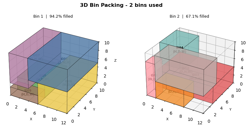
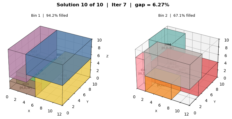
   1  I001, I005, I006, I007, I009        1130   94.2%  I001:(D,W,H), I005:(D,H,W), I006:(W,D,H), I007:(D,H,W), I009:(H,D,W)
   2  I002, I003, I004, I008, I010         805   67.1%  I002:(D,H,W), I003:(W,D,H), I004:(H,D,W), I008:(W,D,H), I010:(D,H,W)

1.3. Visualize and Analyze Results

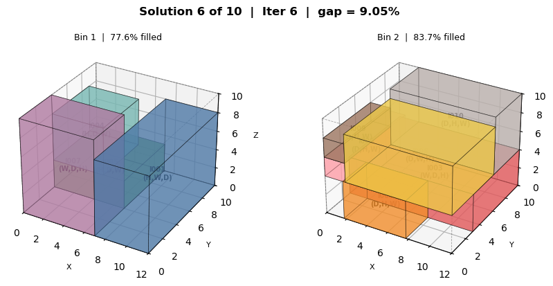
Now that we have a solution, let’s visualize it and extract a few useful analytics using pandas and matplotlib. Each coloured cuboid represents one item placed at its optimized (X, Y, Z) coordinates inside the bin.

COLOR_PALETTE = [
    "#4E79A7", "#F28E2B", "#E15759", "#76B7B2",
    "#59A14F", "#EDC948", "#B07AA1", "#FF9DA7",
    "#9C755F", "#BAB0AC", "#8CD17D", "#D4A6C8",
    "#F1CE63", "#86BCB6", "#E45756"
]
ITEM_COLORS = {i: COLOR_PALETTE[idx % len(COLOR_PALETTE)] for idx, i in enumerate(I)}


def draw_box(ax, x0, y0, z0, w, d, h, color, alpha=0.55):
    """Draw a filled 3D box as a Poly3DCollection."""
    x1, y1, z1 = x0 + w, y0 + d, z0 + h
    faces = [
        [[x0, y0, z0], [x1, y0, z0], [x1, y1, z0], [x0, y1, z0]],  # bottom
        [[x0, y0, z1], [x1, y0, z1], [x1, y1, z1], [x0, y1, z1]],  # top
        [[x0, y0, z0], [x1, y0, z0], [x1, y0, z1], [x0, y0, z1]],  # front
        [[x0, y1, z0], [x1, y1, z0], [x1, y1, z1], [x0, y1, z1]],  # back
        [[x0, y0, z0], [x0, y1, z0], [x0, y1, z1], [x0, y0, z1]],  # left
        [[x1, y0, z0], [x1, y1, z0], [x1, y1, z1], [x1, y0, z1]],  # right
    ]
    ax.add_collection3d(Poly3DCollection(faces, alpha=alpha, facecolor=color, edgecolor='black', linewidth=0.5))


def draw_bin_outline(ax, W, D, H):
    """Draw the bin as a dashed wireframe."""
    for xv in [0, W]:
        for yv in [0, D]:
            ax.plot([xv, xv], [yv, yv], [0, H], 'k--', lw=0.6, alpha=0.35)
    for xv in [0, W]:
        for zv in [0, H]:
            ax.plot([xv, xv], [0, D], [zv, zv], 'k--', lw=0.6, alpha=0.35)
    for yv in [0, D]:
        for zv in [0, H]:
            ax.plot([0, W], [yv, yv], [zv, zv], 'k--', lw=0.6, alpha=0.35)


def plot_packing(packing, positions, orientations, title):
    """Draw each used bin with its items, one subplot per bin."""
    n_cols = min(3, len(packing))
    n_rows = int(np.ceil(len(packing) / n_cols))
    fig = plt.figure(figsize=(4.5 * n_cols, 4 * n_rows))

    for plot_idx, (j, item_list) in enumerate(packing.items()):
        ax = fig.add_subplot(n_rows, n_cols, plot_idx + 1, projection='3d')

        for i in item_list:
            x0, y0, z0 = positions[i]
            w_eff, d_eff, h_eff = eff_dims(i, orientations[i])
            draw_box(ax, x0, y0, z0, w_eff, d_eff, h_eff, color=ITEM_COLORS[i])
            ax.text(x0 + w_eff / 2, y0 + d_eff / 2, z0 + h_eff / 2, f"{i}\n{PERM_LABELS[orientations[i]]}",
                    ha='center', va='center', fontsize=7, fontweight='bold')

        draw_bin_outline(ax, BIN_WIDTH, BIN_DEPTH, BIN_HEIGHT)

        fill = 100.0 * sum(volumes[i] for i in item_list) / BIN_VOLUME
        ax.set_xlim(0, BIN_WIDTH)
        ax.set_ylim(0, BIN_DEPTH)
        ax.set_zlim(0, BIN_HEIGHT)
        ax.set_xlabel('X', fontsize=8)
        ax.set_ylabel('Y', fontsize=8)
        ax.set_zlabel('Z', fontsize=8)
        ax.set_title(f"Bin {j+1}  |  {fill:.1f}% filled", fontsize=9)

    fig.suptitle(title, fontsize=12, fontweight='bold')
    plt.tight_layout()
    plt.show()


plot_packing(packing, positions, orientations, f"3D Bin Packing - {len(packing)} bins used")

# Post-solution analysis with pandas
rows = []
for j, item_list in packing.items():
    vol_used = sum(volumes[i] for i in item_list)
    rows.append({
        "Bin": j + 1,
        "Items": ", ".join(item_list),
        "Volume Used": vol_used,
        "Free Volume": BIN_VOLUME - vol_used,
        "Fill %": round(100.0 * vol_used / BIN_VOLUME, 1),
    })

df_result = pd.DataFrame(rows)
display(HTML(df_result.to_html(index=False)))

print(f"Average bin fill rate : {df_result['Fill %'].mean():.1f}%")
print(f"Total wasted volume   : {df_result['Free Volume'].sum()} units³")

Bin	Items	Volume Used	Free Volume	Fill %
1	I001, I005, I006, I007, I009	1130	70	94.2
2	I002, I003, I004, I008, I010	805	395	67.1

Average bin fill rate : 80.7%
Total wasted volume   : 465 units³

1.4. Callback-Based Extension

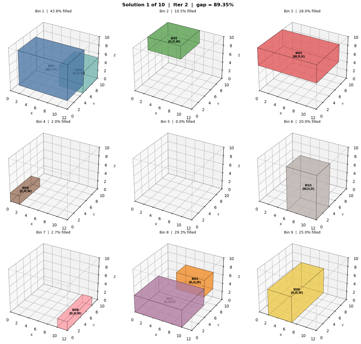
In Notebook 2 we used callbacks in the context of a small MINLP. Here we put two of them to practical use while solving the same model again with build_binpacking_model():

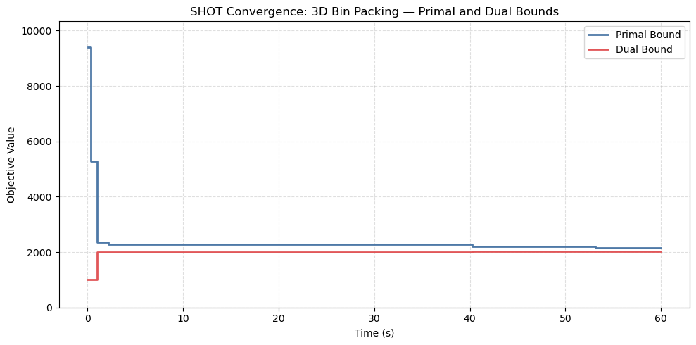
• NewPrimalSolution records every new primal solution, so that we can replay the packings afterwards.

• BoundsUpdated records the primal and dual bounds every time one of them changes, so that we can plot how they converge over time.

# Create solver
solver2 = SHOTpy.Solver()
solver2.updateSetting("Dual.MIP.Solver", int(SHOTpy.MIPSolver.Highs))
solver2.updateSetting("Termination.TimeLimit", 60.0)
solver2.updateSetting("Output.Console.LogLevel", 3)   # Only warnings and errors

# Create problem
problem2, variables2 = build_binpacking_model(solver2)

# Set problem
assert solver2.setProblem(problem2)

# Register callbacks to track the primal solutions and the bounds
primal_log = []
bounds_log = []

def on_new_primal(ctx):
    primal_log.append({
        "iter": ctx.iterationNumber,
        "obj": ctx.objectiveValue,
        "dual": ctx.dualBound,
        "rel_gap_%": 100 * ctx.relativeGap,
        "solution": ctx.point,
    })

def on_bounds_updated(ctx):
    bounds_log.append({"time": ctx.elapsedTime, "primal": ctx.primalBound, "dual": ctx.dualBound})

solver2.registerCallback(SHOTpy.CallbackLocation.NewPrimalSolution, on_new_primal)
solver2.registerCallback(SHOTpy.CallbackLocation.BoundsUpdated, on_bounds_updated)

# Solve
assert solver2.solveProblem()
print(f"Status: {solver2.getModelReturnStatus().name} ({solver2.getTerminationReason().name})")

 Performing bound tightening on original problem.
  - Bounds for 0 variables tightened in 0.00 s and 1 passes.
  - Objective bounds are: [0, 13440]

Status: FeasibleSolution (TimeLimit)

print(f"Primal solutions recorded by NewPrimalSolution: {len(primal_log)}")
print(f"Bound updates recorded by BoundsUpdated       : {len(bounds_log)}\n")
print(f"  {'Iter':>6}  {'Objective':>10}  {'Dual Bound':>12}  {'Gap (%)':>8}")
print(f"  {'-'*6}  {'-'*10}  {'-'*12}  {'-'*8}")
for row in primal_log:
    print(f"  {row['iter']:>6}  {row['obj']:>10.1f}  {row['dual']:>12.1f}  {row['rel_gap_%']:>8.2f}")

Primal solutions recorded by NewPrimalSolution: 10
Bound updates recorded by BoundsUpdated       : 13

    Iter   Objective    Dual Bound   Gap (%)
  ------  ----------  ------------  --------
       2      9392.0        1000.0     89.35
       3      5271.0        1000.0     81.03
       4      2377.0        2000.0     15.86
       4      2359.0        2000.0     15.22
       5      2281.0        2000.0     12.32
       6      2230.1        2028.3      9.05
       6      2203.0        2028.3      7.93
       7      2169.0        2028.3      6.48
       7      2164.0        2028.3      6.27
       7      2164.0        2028.3      6.27

# Convergence plot; the bounds are extended to the end of the solve
df_bounds = pd.DataFrame(bounds_log)
end_time = (solver2.getDoubleSetting("Termination.TimeLimit")
            if solver2.getTerminationReason() == SHOTpy.TerminationReason.TimeLimit else df_bounds["time"].max())
end = {"time": end_time, "primal": solver2.getPrimalBound(), "dual": solver2.getGlobalDualBound()}
df_bounds = pd.concat([df_bounds, pd.DataFrame([end])], ignore_index=True)
df_bounds = df_bounds.replace([np.inf, -np.inf], np.nan)

fig, ax = plt.subplots(figsize=(10, 5))
ax.step(df_bounds["time"], df_bounds["primal"], where="post", linewidth=2, label="Primal Bound", color="#4E79A7")
ax.step(df_bounds["time"], df_bounds["dual"], where="post", linewidth=2, label="Dual Bound", color="#E15759")

ax.set_xlabel("Time (s)")
ax.set_ylabel("Objective Value")
ax.set_title("SHOT Convergence: 3D Bin Packing — Primal and Dual Bounds")
ax.set_ylim(0, 1.1 * df_bounds["primal"].max())
ax.legend()
ax.grid(True, linestyle="--", alpha=0.4)
plt.tight_layout()
plt.show()

# Visualize the 3D packing of the first, an intermediate and the last primal solution
steps = sorted({0, len(primal_log) // 2, len(primal_log) - 1})

for step in steps:
    row = primal_log[step]
    step_packing, step_positions, step_orientations = decode_packing(row["solution"], variables2)
    plot_packing(step_packing, step_positions, step_orientations,
                 f"Solution {step+1} of {len(primal_log)}  |  Iter {row['iter']}  |  gap = {row['rel_gap_%']:.2f}%")

2. Key Takeaways

1. Utilize Your Favorite Python Libraries

You can seamlessly combine SHOTpy with standard Python libraries: pandas handles data loading and postprocessing, numpy provides quick statistics, and matplotlib turns abstract solution vectors into intuitive visual summaries (to name a few). The solver becomes just one component in a larger data workflow.

2. Callbacks Bridge the Solver and Your Application

Callbacks are not just a research tool — they let you instrument any production workflow. In this notebook we used NewPrimalSolution to replay the intermediate packings and BoundsUpdated to plot how the bounds converge. The same pattern works for writing solutions to a database, updating a dashboard, triggering alerts, or feeding results into a downstream pipeline — all without waiting for the full solve to finish. This makes SHOT a first-class citizen in any real-time or iterative decision-support workflow, not just a standalone black box.

3. SHOTpy Enables You to Build More Than Optimization Models

SHOTpy bridges the gap between optimization research and real-world applications. The same Python interface can be used to prototype new ideas, analyze solver performance, build visualizations, and integrate optimization into larger software systems. This flexibility makes SHOTpy a powerful tool for both researchers and practitioners.

Next Steps

In Notebook 4, you’ll learn more about advanced modeling, e.g., how to analyze the functions of a model in Python: evaluating values, gradients and Hessians, bounding them with interval arithmetic, checking convexity numerically, and constructing αBB underestimators.